Excel VBA AutoFilter multiple criteria for Data Range
Learn MS Excel advanced filter option & accessing it from VBA with this simple tutorial. We will cover these topics.
- Excel Menu – To add filter for a range
- Excel VBA Macro code to add multiple criteria to Autofilter.
- VBA to Read visible rows after applying filter.
- VBA code to read selection criteria.
This is applicable for MS Excel 2007 Autofilter or any version above it.
1. How to Use Filter in Excel? – Menu option
To add a filter option, open a Excel workbook with table of data & follow these steps.
- Select the data range or table for which you need to add filter.
- Choose ‘Home’ in Excel menu.
- Select ‘Sort & Filter’ option in ‘Editing’ section.
- Press ‘Filter’. ( shortcut: ‘Alt + H + S + F’)
A drop down will be added at the first row or column header of selected data range or table.
Click on any of the drop down menu & choose a data in it. Data that only matches selection criteria in that column will we displayed and other rows will be hidden. To remove the filter, follow the same steps that we used to add it.
Once we add a filter, we can use it in different combination of scenarios as given below.
- 1 Criteria: Click Filter drop down and enable check box for any one the criteria.
- 2 Criteria: Click filter drop down, then choose “Text Filter” option for adding 2 criteria with logical operators (like equals, contains, greater than, less than etc.,).
- More than 2: Either select each criteria manually from drop down or use VBA code mentioned below.
2. VBA Autofilter with Multiple Criteria
If we have to select more than 2 criteria or even 100s of values in consideration? We need to use some MS Excel advanced filter options or use the code below. With this we can autofilter data from a column using more than 2 selection criteria. The function we are going to use to automate this is:
AutoFilter(Field, Criteria1, Operator, Criteria2, VisibleDropDown)
2.1 Autofilter in Sheet 1 based on Sheet 2 data
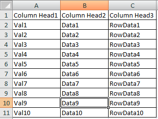
To understand how this works, create new workbook that has Sheet1 with data and Sheet2 with Criteria list as in the Input settings images below.
Data Worksheet (Sheet1) – Input 1
Multiple Criteria (Sheet2) – Input 2
In sheet2 column1 Enter these values
- Val1,
- Val5,
- Val6
2.2 Excel Macro Code to Autofilter data with Criteria list
- Copy the below code and paste it in Excel VB Editor (Press Alt + F11 to view VBE)
- Execute the code by pressing F5.
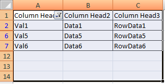
- You will get the Results as shown in Output image.
Option Explicit
Sub Excel_VBA_AutoFilter_Using_Multiple_Criteria_List()
    'Variables Declacaration
    Dim Criteria_Val(100) As String
    Dim iRow As Integer

    'Loop Thru the List and Create Filter Criteria Array
    iRow = 0
    While Sheets(2).Cells(iRow + 1, 1) <> ""
        Criteria_Val(iRow) = Sheets(2).Cells(iRow + 1, 1)
        iRow = iRow + 1
    Wend

    'Multiple Criteria List is Created. Pass it as parameter to Filter
    Sheets(1).Range("A1:A10").AutoFilter Field:=1, Criteria1:=Criteria_Val, Operator:=xlFilterValues
End Sub
2.3 Output of Excel Advanced Filter with Multiple criteria
Once the code is executed, the sheet1 will show output as shown below, displaying only the data that meet the criteria in sheet2.
3. VBA to Read only Visible Data after Excel Filter
Use the below simple for to read the visible data range after a filter is being applied.
Option Explicit
Sub Call_Read_Visible_Range_Function()
    Dim wSht As Worksheet
    Set wSht = ThisWorkbook.Sheets("sheet1")
    If wSht.FilterMode = True Then
        VBA_Read_Visible_Rows 1, 2000, wSht
    End If
End Sub

Public Sub VBA_Read_Visible_Rows(startRow As Long, endRow As Long, wSht As Worksheet)

    '''''Method1 using Rows.Hidden Property'''''
    Dim iRow As Long, iCol As Long
    iCol = 1
    'Loop thru each row and find visible range
    For iRow = startRow To endRow
        If wSht.Rows(iRow).Hidden = False Then
            'Include code here to process visible rows table data
            MsgBox "(1) Read Data in Visible Row : " & wSht.Cells(iRow, iCol)
        End If
    Next iRow

    '''''Method2 using xlCellTypeVisible'''''
    Dim wRng As Range, iRng As Range
    Set wRng = wSht.Range("A" & startRow & ":A" & endRow)
    'Set Visible Range and loop through each cell in visible Range
    For Each iRng In wRng.SpecialCells(xlCellTypeVisible)
        'Enter Code here to read visible range data
        MsgBox "(2) Read Data in Visible Row" & iRng.Address
    Next iRng

End Sub
Since few rows will be hidden once the filter is applied, it is hard to read only the visible data through a macro. This vba macro reads only visible data in the table.
4. Excel VBA to get Autofilter selection Criteria
If we have already done with all the filtering & just want to read criteria list itself, then use the below simple code.
Sub VBA_Read_AutoFilter_Criteria()
    Dim wSht As Worksheet, iCrt As Variant, iFil As Filter, strCri As String
    Dim wRng As Range, iRng As Range, i As Long, j As Long

    'Assign worksheet & range
    Set wSht = ThisWorkbook.Sheets("sheet7")
    Set wRng = wSht.Range("A" & 1 & ":F" & 1)

    'Loop thru all columns with filters & read Criteria details
    For i = 1 To wRng.Parent.AutoFilter.Filters.Count
        Set iFil = wRng.Parent.AutoFilter.Filters(i)
        If iFil.On Then
            Select Case iFil.Operator
                Case xlOr
                    MsgBox "Values " & iFil.Criteria1 & " OR " & iFil.Criteria2

                Case xlAnd
                    MsgBox "Values " & iFil.Criteria1 & " AND " & iFil.Criteria2

                Case xlFilterValues
                    iCrt = iFil.Criteria1
                    'Function to get number of dimentions of a Variant or Array size of a variant
                    For j = 1 To Application.WorksheetFunction.CountA(iCrt)
                        strCri = strCri & "," & iCrt(j)
                    Next j
                    MsgBox "Multiple Criteria Array List: " & strCri

                Case Else
                    MsgBox "Operator Used: " & iFil.Operator
            End Select
        End If
    Next i
End Sub
Note that this macro does not read data, instead it reads and displays on the list applied in criteria. For all possible operators used inside a filter, please check the syntax details in the next section.
MSOffice Excel Macro Autofilter Syntax
We will learn more about the parameters passed to the Excel advanced Filter method.
-
- Field – It is the Column Number which we want to Filter
- Criteria1 – Data or List of Data or Criteria. In the above code, we concatenate the data from criteria list and pass it to the function.
- Operator – In the code we have used xlFilterValues since we filter a list of values from a range.
- xlAnd – Logical AND of Criteria1 and Criteria2.
- xlBottom10Items – Lowest-valued items displayed (number of items specified in Criteria1).
- xlBottom10Percent – Lowest-valued items displayed (percentage specified in Criteria1).
- xlFilterCellColor – Color of the cell
- xlFilterDynamic – Dynamic filter
- xlFilterFontColor – Color of the font
- xlFilterIcon – Filter icon
- xlFilterValues – Filter values
- xlOr – Logical OR of Criteria1 or Criteria2.
- xlTop10Items – Highest-valued items displayed (number of items specified in Criteria1).
- xlTop10Percent – Highest-valued items displayed (percentage specified in Criteria1).
- Criteria2 – If we use any Local AND or OR in Operation, then Criteria 2 is used to compare with Criteria1.
- VisibleDropDown – Set it to True to view Filter Drop down or False to Hide Drop Down.

