Pivot Chart In Excel – How To Create A Pivot Table?

In Excel – What is a Pivot Table?

Pivot Table is used to consolidate or summarize a table with huge volume data.

Pivot table or Pivot chart are very quick powerful tool to view the data in simple format. it has easy to use, drag & drop controls to customize consolidated data.

These Pivot table fields can be customized – table headers, subtotals, grouping data, build chart, filter data etc.,

Pivot Report – Create Report as a Table in Excel

To create a Pivot table in Excel worksheet, use these steps.

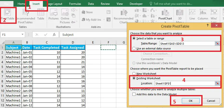
1. Select Table data to be consolidated.
2. Click ‘Insert’ tab in Menu.
3. Choose ‘Pivot Table’ in Tables.
4. Select destination cell to create report.
5. Click ok.

A empty table space for the Pivot table. You can see controls for Pivot table fields on the right hand side. It will list the table fields & other controls. Drag & drop the column headers to any of these section – Filter, Columns, Rows or Values.

What these sections specify? Lets find out.

Pivot Table – Excel Help

• Filters: Once you drop a field header to this section, this means that the table values can be filtered based on this field.
• Columns or Rows: Field headers dropped to this section will be displayed as Row or Column header in Pivot table.
• Values: Fields dropped in this section will be the actual data for pivot table. By default this will show the count of the dropped field. Right click on this field to choose what consolidation you are trying to achieve (like Sum, count, average of data fields.)

This Pivot table option is something that is hard to explain in words. But, it is so easy to use. So, it is better to get your hands dirty. Try to create a pivot table on sample data. Then try multiple options & combinations on this table to learn its full strength.

Add Pivot Chart

To add a Pivot chat to the Excel, follow these steps after creating the pivot table.

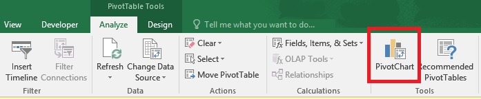
1. Click the Pivot table.
2. In Menu, select Analyze -> Pivot Chart.
3. Select Chart type.
4. Click ‘Ok’.

A Pivot chart will be added to the sheet that you have chosen. It will show the data in chart format.

How To Delete a Pivot Table?

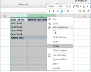
To delete the Pivot table, once you have processed the required analysis. Follow these steps.

1. Select all Columns in Pivot Table.
2. Right Click.
3. Choose Delete.

If you delete only first row or the cell that has Pivot table, Excel will give error message. So, select all the columns and try deleting it.

No matter how much you read about a Pivot table, it is not going to give you enough expertise until you try it.