How to Replace Vlookup NA with 0 or blank in Excel?
In many of the Excel formula, we get “#N/A” as return value. Espcially we get this quite often in lookup, index, match formulas.
If we use a formula like VLOOKUP in a table or report, these error values fills up in many places which spoils the look & feel of the report.
To avoid this, you can replace #N/A with 0, blank or a hyphen in all the occurances with a simple formula trick.
Lets see how to do this with an example …
Table with #N/A Error
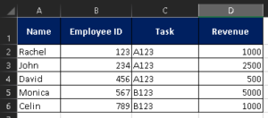
Assume you have a table with employee details & revenue like this:
Now, we apply a vlookup formula from another table to get revenue of each employee by using the name as in this image.
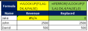
You can see that in the Vlookup we get #N/A error. And in the next column we replace it with a 0 using the IFERROR formula.
Not only a zero, we can even replace it with a “-” (hyphen) that looks appealing or just blank. Both these options will make the report appealing.
Excel Formula to Replace #N/A with 0
Here is little more explanation about this formula.
'// Replacing #N/A with 0 in Excel using Formula.
'   =IFERROR (expression, value-if-error)

=IFERROR(VLOOKUP(2,2,1,FALSE),"0")
' - Display value if no error
' - Display 0 if error

'//Replace #N/A with blank
=IFERROR(VLOOKUP(2,2,1,FALSE),"")
This IFERROR function also handles #VALUE, #NAME, #DIV/0 errors. Almost any error is handled by this function and you can replace the correspoding error with any value of your choice.
There is also another function with a slight variation is available. It is ISNA. This function cannot be used directly to replace a return value, but can be used to detect the error.
Meaning this function will return TRUE if the expression within it is an error value. Read this topic to know more about the #N/A & other error handling formula.
Additional Readin:
- Different methods available to remove N/A Error in Vlookup.
- How to generate a N/A error in Excel.
External Resource:
- Here is another topic that discusses the same in detail.